The hare and the turtle: why agile approaches are often not feasible in applied psychology
Author
Gjalt-Jorn Peters
Published
March 9, 2019
Recently, a case study was published where the usefulness of agile methods in developing behavior change interventions was explored (Ploos van Amstel, Heemskerk, Renes & Hermsen, 2017, doi:10.1080/14606925.2017.1353014). Although such approaches can have an added value, in the context of applied psychology this added value can quickly become a dangerous pitfall. In this brief blog post I explain why, and how to avoid it.
Basics of Agile approaches
Agile approaches first became popular in software development, quickly gaining ground after publication of the ‘Manifesto for Agile Software Development’ published in 2001 (http://agilemanifesto.org/). Where ‘traditional’ methods are often linear, characterised by a phase of thorough planning that is followed by a phase of executing those plans, Agile methods denounce such meticulous planning in favour of an iterative approach, where the execution starts almost immediately based on a first rough draft. The product is then evaluated and adjusted in cycles that quickly succeed each other.
Agile behavior change
Applied to behavior change, agile methods prompt rapid development of a first working version of an intervention. This means that common preliminary steps, such as conducting a needs assessment and doing literature research and qualitative and quantitative research to identify the most important determinants of the target behavior, are often foregone. This first working version is then evaluated, and on the basis of this evaluation, it can be improved into a next version. This process can be repeated as resources (time and money) allow.
To enable this, you need to know what to improve. This means you need to collect information about which aspects of your intervention work and which don’t. For example, you could measure the effect it has on a set of determinants that might be important for the target behavior. Alternatively, you need to have an estimate of the intervention’s effect on behavior, and then use an approach akin to the ‘A/B tests’ used in online persuasion to compare multiple alternative interventions to each other.
At first glance, this can seem like a feasible, even exciting approach. It certainly more action-driven and ‘sexy’ that the conventional approaches to behavior change, which require comprehensive canvassing of the literature, talking to your target population extensively, then verifying the preliminary results in quantitative research, and then using complicated-sounding approaches such as Confidence Interval-Based Estimation of Relevance to select the determinants to target (see e.g. doi:10.3389/fpubh.2017.00165).
However…
The pitfall
The pitfall of agile methods as employed in applied psychology relates to the sampling distribution of effect sizes. Decisions that are taken in between the iterations that are central to agile approaches are based on the evaluation of the intervention. To enable improving the intervention in these successive iterations, these decisions require learning about the intervention’s effectiveness from the last iteration. This is inevitably a matter of causality, and therefore, requires an experimental design.
The effect size commonly used in experimental designs is Cohen’s \(d\). Cohen’s \(d\)’s sampling distribution is very wide compared to that of, for example, Pearson’s \(r\) (see doi:10.31234/osf.io/cjsk2). Because one image is worth a thousand words, behold Figure 1.
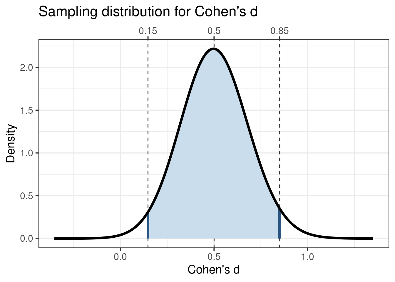
attr(ufs::cohensdCI(d=0.5, n=128, plot=TRUE),'plot') + ggplot2::xlab("Cohen's d") + ggplot2::ylab("Density") + ggplot2::ggtitle("Sampling distribution for Cohen's d") + ggplot2::theme_bw(base_size =15) + ggplot2::theme(axis.title.x.top =element_blank());
Cohen’s d’s sampling distribution for a moderate population effect size (d = 0.5) and for a 2-cell design with 80% power (i.e. 64 participants per group).
This figure shows how wide the sampling distribution of Cohen’s \(d\) is in an experiment with a 2-cell design and 64 participants in each group (i.e. the required sample size to achieve 80% power in a null hypothesis significance testing situation). In this case, obtaining a Cohen’s \(d\) of 0.20 of 0.25 is very likely. If a Cohen’s \(d\) of 0.5 is obtained, this means that population values of 0.25 is quite plausible; if a Cohen’s \(d\) of .25 is obtained, that means that a negative population value for Cohen’s \(d\) is quite likely. For example, let us assume the first iteration of an intervention has a small effect of (Cohen’s \(d\) = 0.2). In that case, this is the sampling distribution it comes from:
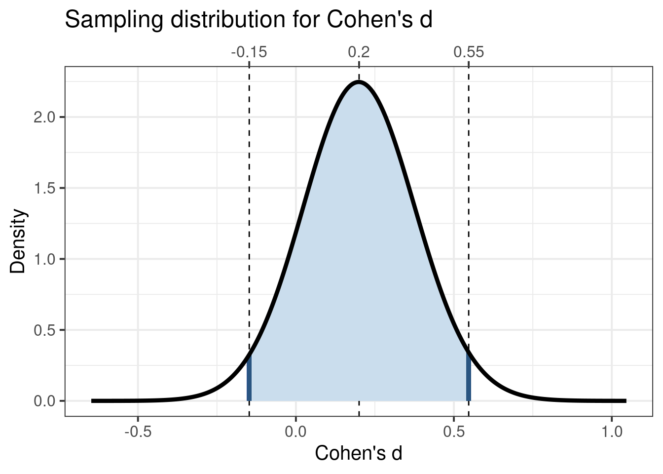
attr(ufs::cohensdCI(d=.2, n=128, plot=TRUE),'plot') + ggplot2::xlab("Cohen's d") + ggplot2::ylab("Density") + ggplot2::ggtitle("Sampling distribution for Cohen's d") + ggplot2::theme_bw(base_size =15) + ggplot2::theme(axis.title.x.top =element_blank());
Cohen’s d’s sampling distribution for a small population effect size (d = 0.2) and for a 2-cell design with 80% power (i.e. 64 participants per group).
In every study (every sample), one Cohen’s \(d\) value is taken randomly from this distribution. The probability that you’ll get a significant result is very low, of course. But even if you do get a significant result (conform NHST), you’ll still not know how effective your intervention is. The point estimate you obtain in any given sample is useless given how wide this sampling distribution is. Therefore, you’ll need the confidence interval to say something useful about how effective that iteration of the intervention is - but that’s extremely wide. You cannot reasonably assume that the population effect is in the middle of the confidence interval, given that they ‘jump around’ (see e.g. https://rpsychologist.com/d3/CI/).
Therefore, with wide confidence intervals, you will learn nothing from one iteration in your agile behavior change approach. This means that you hvae no information to inform your next iteration. This is especially problematic because unless you do invest in comprehensive planning (effectively taking much of the agile out of your agile approach), the first intervention you develop will have a low effect size (the \(d\) = 0.2 is not unreasonable in that case).
Avoiding the pitfall
There is one way to avoid this pitfall: plan your data collection for each iteration such that you obtain sufficiently narrow confidence intervals so that you are able to make informed decisions, thereby enabling iterate towards more effective interventions.
In our preprint about planning for Cohen’s \(d\) confidence intervals (doi:10.31234/osf.io/cjsk2), we introduce functions and provide tables to plan for specific confidence intervals widths. For 95% confidence intervals, this is one of those tables:
Table 1: The required sample sizes for confidence intervals of varying widths with 95% confidence.
0.05
0.1
0.15
0.2
0.25
0.3
0.35
0.4
0.45
0.5
0.2
6178
1545
687
387
248
172
127
97
77
62
0.5
6339
1585
705
397
254
177
130
100
79
64
0.8
6639
1660
738
416
266
185
136
104
83
67
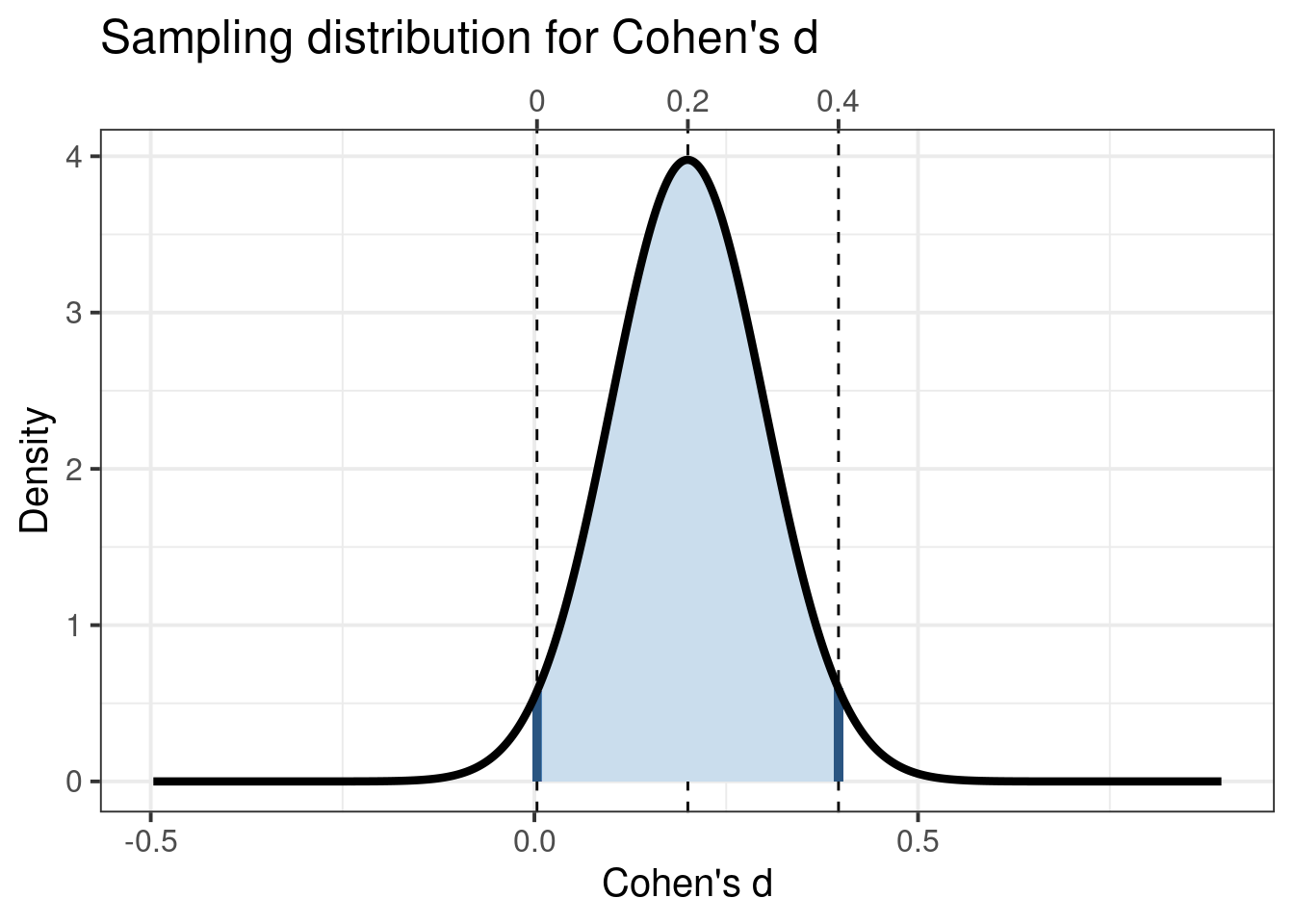
As this table makes clear, 95% confidence intervals for Cohen’s \(d\) only start to become narrower with 200 participants per group. In fact, with 200 participants per group, this is your sampling distribution if the Cohen’s \(d\) for your intervention has a population value of .2:
attr(ufs::cohensdCI(d=.2, n=400, plot=TRUE),'plot') + ggplot2::xlab("Cohen's d") + ggplot2::ylab("Density") + ggplot2::ggtitle("Sampling distribution for Cohen's d") + ggplot2::theme_bw(base_size =15) + ggplot2::theme(axis.title.x.top =element_blank());
Cohen’s d’s sampling distribution for a small population effect size (d = 0.2) and for a 2-cell design with 200 participants per group.
As you see, in that case, it’s still quite likely that you’ll end up with a Cohen’s \(d\) that is very close to zero. You’ll need to get to a total of 1500 participants to get an accurate estimate:
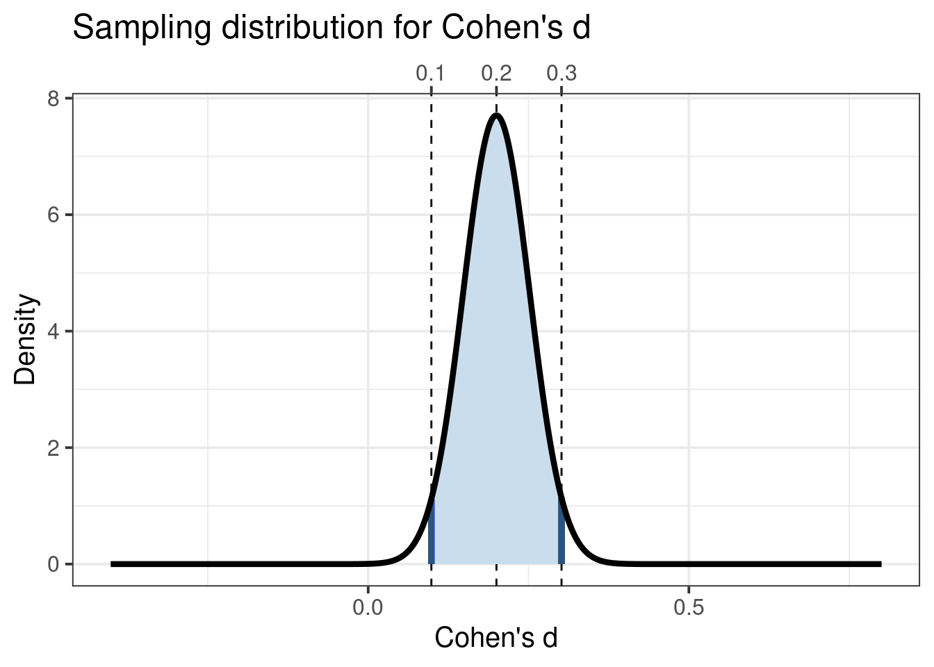
attr(ufs::cohensdCI(d=.2, n=1500, plot=TRUE),'plot') + ggplot2::xlab("Cohen's d") + ggplot2::ylab("Density") + ggplot2::ggtitle("Sampling distribution for Cohen's d") + ggplot2::theme_bw(base_size =15) + ggplot2::theme(axis.title.x.top =element_blank());
Cohen’s d’s sampling distribution for a small population effect size (d = 0.2) and for a 2-cell design with 750 participants per group.
So, for your first iteration to be more or less informative and allow you to improve the intervention in the right direction in the second iteration, you would need around 1500 participants. That’s a lot though - especially given that participants are a scarce resource that you shouldn’t lightly ‘use up’. Even if you can, collecting so much data can cost a lot of time, making it hard to fit in an agile workflow.
Scenarios where agile approaches are feasible
Of course, agile approaches can still be feasible in some situations. Specifically, situations where you can collect data on interventions’ effectiveness without actually requiring participants - instead using publicly available data, for example, by coding people’s behavior in a public space.
However, this narrow field of application is important to keep in mind. If you work with a behavior that cannot be observed in public spaces, you cannot compare alternative initial interventions using an A/B-test like approach. Also, when you want to base the iterative intervention improvements on which components work better and which work worse, you will need to measure your participants’ determinants. In such cases, agile approaches are only feasible if you can afford to test thousands of participants.
In such scenario’s, it quickly becomes faster and cheaper to invest more time and effort in the planning phase and forego an agile approach. An additional complication may be ethical approval - how ethical is it to consume hundreds or thousands of participant-hours more than is necessary if you use another route?
Final notes
I did not write this blog post because I think agile approaches are not useful or valuable; instead, I wrote this because I know that most people don’t normally think from the perspective of sampling distributions, and that can easily lead people to erreoneously believe that agile approaches are widely applicable.
A second remark is that these dynamics (the number of participants, or more accurately, data points, required to obtain more or less stable effect size estimates) do not specifically plague agile approaches. This applies to all research: also, for example, effect evaluations of interventions. If you find this interesting, see our preprint at doi:10.31234/osf.io/cjsk2.